Surface computing, move over!

For a few weeks now, my two team-mates at work and I have been using a “horizontal” whiteboard, lying across the desk surface between us. I had been wanting to try this for a while, but it wasn’t possible because of our previous desk arrangement. Now that we have this large area of space between us and no partitions, this small whiteboard fits perfectly without getting in the way.

We’ve found ourselves using it virtually every day, illustrating explanations, walking through calculations and brainstorming design ideas. Visitors will intuitively pick up a pen and start using the whiteboard when explaining things. It somehow seems to invite people to use it more than most whiteboards. However, it’s not only a collaborative tool: it also makes a great scratch-pad when you’re brainstorming on your own. To ensure that it stays useful, we make an effort to keep the board clean; nothing tends to stay on there for longer than a day or so.

Overall, it’s being used far more than any wall-mounted whiteboards we’ve had near us, and I think this is due to two key differences to wall-mounted boards. Firstly, each one of us can reach the board very easily without having to get up. You just turn your chair slightly and there it is. Secondly, the whiteboard is between us, so it feels less like a presentation aid and more like a collaborative work surface, accessible equally well from all sides.

If your work involves collaborative problem-solving, and if your desk arrangement allows it, I highly recommend setting up a whiteboard like this. Don’t make it too big, because you won’t be able to reach all corners and it will also eat into your desk real-estate. I think ours is 90×60 cm, which is just right. I also recommend investing in some pens with a finer tip than the standard ones you tend to get. Those are designed to be visible from a few meters away, but you’ll find them too thick for handwriting at a comfortable size for close-up work. Edding do quite a range of dry-erase board markers.

Neutech desktop background redux

There was once an appearance theme for Mac OS 8 and 9 called Neutech, by Flanksteak Design. I don't think I particular liked the theme as a whole, but it included a desktop background that has been my favourite background for the last eight years or so since I discovered it:

Here's a detail:

I have made sure I that I always have a copy, which has survived across all the different Macs I've used since. However, the image is only 1024 × 768 pixels, which wasn't small at the time, but makes the image look rather pixelated and blurry on modern displays. I have made several attempts in the past to reproduce it in Photoshop, but never got very far. Today, I sat down again with renewed determination and finally found the secret recipe to emulate the look of the original:

One thing that really helped here was Photoshop CS3's Smart Filters, because I could experiment and keep tweaking the many effects I had to apply. This also means that I can easily produce updated versions in the future as screen resolutions increase.

For the time being, here's a 2560 × 1600 version.

Update: I've changed the grid to look more like dried earth and less like reptile skin, and made minor changes to shading.

Namely 2.5

Sorry to be late by a week or so, but there are several reasons why I didn't get a Leopard-compatible update to Namely out sooner.

First of all, I didn't have Leopard any earlier than most of you; I bought it on Friday the 26th of October at the Apple Store on Regent Street. That's because unlike many Mac developers who dedicate a lot more time to this stuff and who have an income from it, I don't have a Select membership with the Apple Developer Connection.

Secondly, I decided to try out Leopard's improved support for application launching through Spotlight before putting any effort into updating Namely. Ever since Scott Forstall had hinted at this feature at the World-Wide Developers' Conference in 2006, I had been feeling a bit anxious about Leopard rendering Namely redundant. (I generally think it's a good thing when Apple fills a gap that was identified and addressed by third-party developers, but nevertheless, we do tend to fall in love with our applications.) My verdict: Spotlight is not bad, but it didn't win me over. I didn't spend enough time with it to figure out how clever it is about choosing between candidate matches (it seems to at least take into account which app you chose last time), but long enough to find a few things that I didn't like about it:

1. A lot of stuff happens visually in the Spotlight menu, which distracts from your main task: quickly identifying the application you want to launch.
   
2. The icons of listed apps don't always appear straightaway.


3. It only shows three matches, so it's effectively a bit less tolerant.

I guess these things shouldn't be an issue if you only occasionally need an application that's not in your Dock. Finding it through Spotlight will still be much faster than navigating to it in the Finder. But I think that if you use Namely (or, for that matter, any other keyboard-based launcher) for most of your application launching, anything that isn't super-fast isn't fast enough. When I launch an application, I don't want to think much, and I don't want to see much. I just want to launch it. Although Namely's sorting isn't perfectly predictable because it adapts over time, it stabilises quickly enough so you can be pretty confident about what it will suggest when you type something.

The third reason for the delay is that I just wasn't sure what to release. I have been (slowly) working on Namely 3.0, which is controlled through a preference pane and doesn't show up in the Dock. So I was considering finishing that off rather than releasing another update to Namely 2.x. However, I wasn't confident that I could get Namely 3 finished and stable within a few days, so I decided to push out a minor update in the meantime.

Here it is. Annoyingly, I couldn't find a way to make it work on both 10.3.9/10.4 and 10.5 (I link against the 10.5 libraries in order to support Spaces, but this seems to stop Apple's secret application-listing function from working on 10.4), so I had to leave version 2.1 available as a separate download.

Coupland and Helvetica

Douglas Coupland last night at the Bloomsbury theatre in London (at what he said was probably his last ever book reading):

...and someone said making a film about Helvetica is like making a film about off-white paint.

I think in Helvetica. I love Helvetica.

For more of his thoughts on the typeface, also see this piece in the New York Times.

Making sense of standard deviation

I love the feeling of getting to understand a seemingly abstract concept in intuitive, real-world terms. It means you can comfortably and freely use it in your head to analyse and understand things and to make predictions. No formulas, no paper, no Greek letters. It’s the basis for effective analytical thinking. The best measure of whether you’ve “got it” is how easily you can explain it to someone and have them understand it to the same extent. I think I recently reached that point with understanding standard deviation, so I thought I’d share those insights with you.

Standard deviation is one of those very useful and actually rather simple mathematical concepts that most people tend to sort-of know about, but probably don’t understand to a level where they can explain why it is used and why it is calculated the way it is. This is hardly surprising, given that good explanations are rare. The Wikipedia entry, for instance, like all entries on mathematics and statistics, is absolutely impenetrable.

First of all, what is deviation? Deviation is simply the “distance” of a value from the mean of the population that it’s part of:

Now, it would be great to be able to summarise all these deviations with a single number. That’s exactly what standard deviation is for. But why don’t we simply use the average of all the deviations, ignoring their sign (the mean absolute deviation or, simply, mean deviation)? That would be quite easy to calculate. However, consider the following two variables (for simplicity, I will use data sets with a mean of zero in all my examples):

There’s obviously more variation in the second data set than in the first, but the mean deviation won’t capture this; it’s 2 for both variables. The standard deviation, however, will be higher for the second variable: 2.24. This is the crux of why standard deviation is used. In finance, it’s called volatility, which I think is a great, descriptive name: the second variable is more volatile than the first. [Update: It turns out I wasn't being accurate here. Volatility is the standard deviation of the changes between values – a simple but significant difference.] Dispersion is another good word, but unfortunately it already has a more general meaning in statistics.

Next, let’s try to understand why this works; that is, how does the calculation of standard deviation capture this extra dispersion on top of the mean deviation?

Standard deviation is calculated by squaring all the deviations, taking the mean of those squares and finally taking the square root of that mean. It’s the root-mean-square (RMS) deviation (N below is the size of the sample):

RMS Deviation = √(Sum of Squared Deviations / N)

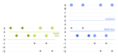
Intuitively, this may sound like a redundant process. (In fact, some people will tell you that this is done purely to eliminate the sign on the negative numbers, which is nonsense.) But let’s have a look at what happens. The green dots in the first graph below are the absolute deviations of the grey dots, and the blue dots in the second graph are the squared deviations:

The dotted blue line at 5 is the mean of the squared deviations (this is known as the variance). The square root of that is the RMS deviation, lying just above 2. Here you can see why the calculation works: the larger values get amplified compared to the smaller ones when squared, “pulling up” the resulting root-mean-square.

That’s mostly all there’s to it, really. However, there’s one more twist to calculating standard deviation that is worth understanding.

The problem is that, usually, you don’t have data on a complete population, but only on a limited sample. For example, you may do a survey of 100 people and try to infer something about the population of a whole city. From your data, you can’t determine the true mean and the true standard deviation of the population, only the sample mean and an estimate of the standard deviation. The sample values will tend to deviate less from the sample mean than from the true mean, because the sample mean itself is derived from, and therefore “optimised” for, the sample. As a consequence, the RMS deviation of a sample tends to be smaller than the true standard deviation of the population. This means that even if you take more and more samples and average their RMS deviations, you will not eventually reach the true standard deviation.

It turns out that to get rid of this so-called bias, you need to multiply your estimate of the variance by N/(N-1). (This can be mathematically proven, but unfortunately I have not been able to find a nice, intuitive explanation for why this is the correct adjustment.)

For the final formula, this means that instead of taking a straightforward mean of the squared deviations, we sum them and divide by the sample size minus 1:

Estimated SD = √(Sum of Squared Deviations / (N - 1))

You can see how this will give you a slightly higher estimate than a straight root-mean-square, and how the larger the sample size, the less significant this adjustment becomes.

Update: Some readers have pointed out that using the square to "amplify" larger deviations seems arbitrary: why not use the cube or even higher powers? I'm looking into this, and will update this article once I've figured it out or if my explanation turns out to be incorrect. If anybody who understands this better than me can clarify, please leave a comment.

On pie charts etc.

On the subject of pie charts, information design god Edward Tufte has the following to say in The Visual Display of Quantitative Information:

A table is nearly always better than a dumb pie chart […]. Given their low data-density and failure to order numbers along a visual dimension, pie charts should never be used.

Although I tried for some time to convince myself and others that this is true, I have failed to come up with a really convincing argument against using pie charts. In fact, I have decided that they aren’t useless at all. Consider the following data, shown as a table, a pie chart, a bar chart and a stacked bar:

One basic feature of all the graphical representations is that they give an immediate impression about which are large and which are small contributors. The table, on the other hand, has no physical attribute that is analogous to quantity. Instead, you need to read and interpret the arbitrary symbols we use for numbers, form a more conceptual representation of the quantities in your head and compare them. You can get around this by ordering the table by value, but you’ll lose the original ordering of the items.

With regards to precision, the table obviously wins. The bar chart also offers pretty good precision as long as you don’t make it too small. The stacked bar may seem to have the upper hand over the pie chart because it has a scale, but reading values isn’t as easy as you may think. Only the first and last section are reliably easy to read. For all the sections in between, the grid lines are of little help. For example, can you confidently say at a glance whether the red section represents more or less than 50%? In the pie chart, you can at least tell straightaway that A contributes slightly over a quarter, B more than half and C around one eighth. And often that’s all you want to know. Do you really care whether an item contributes 27% or 29%? (I’m not saying that you don’t, only that that’s a question to ask when deciding what representation to use).

The stacked bar is also pretty impossible to label (no, legends are not a satisfactory solution). However, this can also be true for pie charts, especially if there are many segments and/or if they have long titles.

A further restriction of pie charts is that they don’t allow adding a further dimension to provide comparisons between different sets of data. Multiple pie charts shown side by side aren’t really comparable, because the whole structure of each pie will be different. This is where tables or bar charts can do much better.

In summary, I’d like to suggest the following guidelines for using pie charts:

1. Use them if you want to give a high-level impression of the distribution of proportions.
2. Don’t use them if precision is important, or include numbers if you have space.
3. Don’t use them if order is important.
4. Don’t use them if you need to show multiple data sets, e.g., changes over time.
5. Keep labels short. Legends suck.
6. If the context allows, use colours that are familiar to the viewer, and use them consistently.

Lastly, I’d like to briefly address the recently fashionable “pixel charts”. Although it’s a terrible waste of time, really. I mean, come on:

In case you still have doubts: the four areas in the following chart are all the same size:

Or are they different sizes? I’m not sure, and I can’t be bothered to count right now.

Clickable control labels for the web

One of my pet peeves in web interfaces has always been that on radio buttons and checkboxes, only the small button itself is clickable. In native Mac and Windows interfaces, you can usually click on the text labels of these controls as well, giving you a much larger target, which, in accordance with Fitts' Law, makes them faster to hit.

Many, or perhaps most, people would probably never notice this difference in behaviour because they have only ever tried clicking on the button proper; the text doesn't visually suggest that it's clickable. But for those of us who are used to this shortcut, the standard web behaviour will catch us out every time. (Actually, I've started to wonder whether I'm the only person on the planet to click on the text labels, since I've never heard anyone else complain about this issue.)

Until a few months ago, I thought this was all just an unfortunate but inevitable limitation of HTML, and that developers found it too much hassle to implement a workaround in JavaScript. Then, I discovered HTML's label element. If you mark up a piece of text as a label and set its for attribute to be the ID of a form control, it becomes the "official" label for that control. The practical effect of this is that in most browsers, clicking the label will actually do something useful. For checkboxes and radio buttons, it will toggle their state, while for text fields, it will put the focus on the field. This works in Internet Explorer 6(!) and 7, Safari (I only checked version 3.0.2), Firefox and Camino. OmniWeb will do it in the upcoming 5.6 release.

So code like the following:

<input
 type="radio"
 name="os"
 id="mac"
 value="mac">
<label
 for="mac">Mac user</label>

<input
 type="radio"
 name="os"
 id="windows"
 value="windows">
<label
 for="windows">Windows user</label>

<input
 type="checkbox"
 name="loving_it"
 id="loving_it">
<label
 for="loving_it">And loving it</label>

results in nice, fully clickable controls like this:

Mac user Windows user And loving it

There's also an alternative, simpler syntax that doesn't require using the for and id attributes. Instead, you can just make the label element a parent of the control:

<label>
  <input
   type="radio"
   name="os"
   value="mac">Mac user
</label>

However, this does not work in Internet Explorer 6, so if you want to be inclusive, stick with the more explicit syntax.