I love the feeling of getting to understand a seemingly abstract concept in intuitive, real-world terms. It means you can comfortably and freely use it in your head to analyse and understand things and to make predictions. No formulas, no paper, no Greek letters. It’s the basis for effective analytical thinking. The best measure of whether you’ve “got it” is how easily you can explain it to someone and have them understand it to the same extent. I think I recently reached that point with understanding standard deviation, so I thought I’d share those insights with you.
Standard deviation is one of those very useful and actually rather simple mathematical concepts that most people tend to sort-of know about, but probably don’t understand to a level where they can explain why it is used and why it is calculated the way it is. This is hardly surprising, given that good explanations are rare. The Wikipedia entry, for instance, like all entries on mathematics and statistics, is absolutely impenetrable.
First of all, what is deviation? Deviation is simply the “distance” of a value from the mean of the population that it’s part of:

Now, it would be great to be able to summarise all these deviations with a single number. That’s exactly what standard deviation is for. But why don’t we simply use the average of all the deviations, ignoring their sign (the mean absolute deviation or, simply, mean deviation)? That would be quite easy to calculate. However, consider the following two variables (for simplicity, I will use data sets with a mean of zero in all my examples):

There’s obviously more variation in the second data set than in the first, but the mean deviation won’t capture this; it’s 2 for both variables. The standard deviation, however, will be higher for the second variable: 2.24. This is the crux of why standard deviation is used. In finance, it’s called volatility, which I think is a great, descriptive name: the second variable is more volatile than the first. [Update: It turns out I wasn't being accurate here. Volatility is the standard deviation of the changes between values – a simple but significant difference.] Dispersion is another good word, but unfortunately it already has a more general meaning in statistics.
Next, let’s try to understand why this works; that is, how does the calculation of standard deviation capture this extra dispersion on top of the mean deviation?
Standard deviation is calculated by squaring all the deviations, taking the mean of those squares and finally taking the square root of that mean. It’s the root-mean-square (RMS) deviation (N below is the size of the sample):
RMS Deviation = √(Sum of Squared Deviations / N)
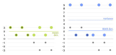
Intuitively, this may sound like a redundant process. (In fact, some people will tell you that this is done purely to eliminate the sign on the negative numbers, which is nonsense.) But let’s have a look at what happens. The green dots in the first graph below are the absolute deviations of the grey dots, and the blue dots in the second graph are the squared deviations:

The dotted blue line at 5 is the mean of the squared deviations (this is known as the variance). The square root of that is the RMS deviation, lying just above 2. Here you can see why the calculation works: the larger values get amplified compared to the smaller ones when squared, “pulling up” the resulting root-mean-square.
That’s mostly all there’s to it, really. However, there’s one more twist to calculating standard deviation that is worth understanding.
The problem is that, usually, you don’t have data on a complete population, but only on a limited sample. For example, you may do a survey of 100 people and try to infer something about the population of a whole city. From your data, you can’t determine the true mean and the true standard deviation of the population, only the sample mean and an estimate of the standard deviation. The sample values will tend to deviate less from the sample mean than from the true mean, because the sample mean itself is derived from, and therefore “optimised” for, the sample. As a consequence, the RMS deviation of a sample tends to be smaller than the true standard deviation of the population. This means that even if you take more and more samples and average their RMS deviations, you will not eventually reach the true standard deviation.
It turns out that to get rid of this so-called bias, you need to multiply your estimate of the variance by N/(N-1). (This can be mathematically proven, but unfortunately I have not been able to find a nice, intuitive explanation for why this is the correct adjustment.)
For the final formula, this means that instead of taking a straightforward mean of the squared deviations, we sum them and divide by the sample size minus 1:
Estimated SD = √(Sum of Squared Deviations / (N - 1))
You can see how this will give you a slightly higher estimate than a straight root-mean-square, and how the larger the sample size, the less significant this adjustment becomes.
Update: Some readers have pointed out that using the square to "amplify" larger deviations seems arbitrary: why not use the cube or even higher powers? I'm looking into this, and will update this article once I've figured it out or if my explanation turns out to be incorrect. If anybody who understands this better than me can clarify, please leave a comment.